Regression Analysis in Machine Learning

What is Regression Analysis?

In machine learning, regression analysis is a statistical technique that predicts continuous numeric values based on the relationship between independent and dependent variables. The main goal of regression analysis is to plot a line or curve that best fit the data and to estimate how one variable affects another.

Regression analysis is a fundamental concept in machine learning and it is used in many applications such as forecasting, predictive analytics, etc.

In machine learning, regression is a type of supervised learning. The key objective of regression-based tasks is to predict output labels or responses, which are continuous numeric values, for the given input data. The output will be based on what the model has learned in the training phase.

Basically, regression models use the input data features (independent variables) and their corresponding continuous numeric output values (dependent or outcome variables) to learn specific associations between inputs and corresponding outputs.

Terminologies Used in Regression Analysis

Let us understand some basic terminologies used in regression analysis before going into further detail. The following are some important terminologies −

• Independent Variables − These variables are used to predict the value of the dependent variable. These are also called predictors. In dataset, these are represented as features.
• Dependent Variables − These are the variables whose values we want to predict. These are the main factors in regression analysis. In dataset, these are represented as target variables
• Regression line − It is a straight line or curve that a regressor plots to fit the data points best.
• Overfitting and underfitting − Overfitting is when the regression model works well with the training dataset but not with the testing dataset. It’s also referred to as the problem of high variance. Underfitting is when the model doesn’t work well with training datasets. It’s also referred to as the problem of high bias.
• Outliers − These are data points that don’t fit the pattern of the rest of the data. They are the extremely high or extremely low values in the data set.
• Multicollinearity − multicollinearity occurs when independent variables (features) have dependency among them.

Explore our latest online courses and learn new skills at your own pace. Enroll and become a certified expert to boost your career.

How does Regression Work?

Regression in machine learning is a supervised learning. Basically, regression is a statistical technique that finds a relationship between dependent and independent variables. To implement regression in machine learning, a regression algorithm is trained with a labeled dataset. The dataset contains features (independent variables) and target values (dependent variable).

During the training phase, the regression algorithm learns the relation between independent variables (predictors) and dependent variables (target).

The regression models predict new values based on the learned relation between predictors and targets during the training.

Types of Regression in Machine Learning

Generally, the classification of regression methods is done based on the three metrics &minus: the number of independent variables, type of dependent variables, and shape of the regression line.

There are numerous regression techniques used in machine learning. However, the following are commonly used types of regression −

• Linear Regression
• Logistic Regression
• Polynomial Regression
• Lasso Regression
• Ridge Regression
• Decision Tree Regression
• Random Forest Regression
• Support Vector Regression

Let’s discuss each type of regression in machine learning in detail.

1. Linear Regression

Linear regressions are the most commonly used regression models in machine learning. Linear regression may be defined as the statistical model that analyzes the linear relationship between a dependent variable with a given set of independent variables. A linear relationship between variables means that when the value of one or more independent variables changes (increase or decrease), the value of the dependent variable will also change accordingly (increase or decrease).

Linear regression is further divided into two subcategories: simple linear regression and multiple linear regression (also known as multivariate linear regression).

In simple linear regression, a single independent variable (or predictor) is used to predict the dependent variable.

Mathematically, the simple linear regression can be represented as follows −

Y=mX+bY=mX+b

Where,

• Y is the dependent variable we are trying to predict.
• X is the dependent variable we are using to make predictions.
• m is the slope of the regression line, which represents the effect X has on Y.
• b is a constant known as the Y-intercept. If X = 0, Y would be equal to b.

In multi-linear regression, multiple independent variables are used to predict the dependent variables.

We will learn linear regression in more detail in upcoming chapters.

2. Logistic Regression

Logistic regression is a popular machine learning algorithm used for predicting the probability of an event occurring.

Logistic regression is a generalized linear model where the target variable follows a Bernoulli distribution. Logistic regression uses a logistic function or logit function to learn a relationship between the independent variables (predictors) and dependent variables (target).

It maps the dependent variable as a sigmoid function of independent variables. The sigmoid function produces a probability between 0 and 1. The probability value is used to estimate the dependent variable’s value.

It is mostly used in binary classification problems, where the target variable is categorical with two classes. It models the probability of the target variable given the input features and predicts the class with the highest probability.

3. Polynomial Regression

Polynomial Linear Regression is a type of regression analysis in which the relationship between the independent variable and the dependent variable is modeled as an n-th degree polynomial function. Polynomial regression allows for a more complex relationship between the variables to be captured, beyond the linear relationship in Simple and Multiple Linear Regression.

Polynomial regression is one of the most widely used non-linear regressions. It is very useful because it can model non-linear relationships between predictors and targets, and also it is more sensitive to outliers.

4. Lasso Regression

Lasso regression is a regularization technique that uses a penalty to prevent overfitting and improve the accuracy of regression models. It performs L1 regularization. It modifies the loss function by adding the penalty (shrinkage quantity) equivalent to the summation of the absolute value of coefficients.

Lasso regression is often used to handle high dimensional and high correlation data.

5. Ridge Regression

Ridge regression is a statistical technique used in machine learning to prevent overfitting in linear regression models. It is used as a regularization technique that performs L2 regularization. It modifies the loss or cost function by adding the penalty (shrinkage quantity) equivalent to the square of the magnitude of coefficients.

Ridge regression helps to reduce model complexity and improve prediction accuracy. It is useful in developing many parameters with high weights. It is also well suited to datasets with more feature variables than a number of observations.

It also corrects the multicollinearity in regression analysis. Multicollinearity occurs when independent variables are dependent on each other.

6. Decision Tree Regression

Decision tree regression uses the decision tree algorithm to predict numerical values. The decision tree algorithm is a supervised machine learning algorithm that can be used for both classification and regression.

It is used to predict numerical values or continuous variables. It works by splitting the data into smaller subsets based on the values of the input features and assigning each subset a numerical value. So incrementally, it develops a decision tree

The tree fits local linear regressions that approximate a curve, and each leaf represents a numeric value. The algorithm tries to reduce the mean square error at each child node, which measures how much the predictions deviate from the original target.

The decision tree regression can be used in predicting stock prices or customer behavior etc.

7. Random Forest Regression

Random forest regression is a supervised machine learning algorithm that uses an ensemble of decision trees to predict continuous target variables. It uses a bagging technique that involves randomly selecting subsets of training data to build smaller decision trees. These smaller models are combined to form a random forest model that outputs a single prediction value.

The technique helps improve accuracy and reduce variance by combining the predictions from multiple decision trees.

8. Support Vector Regression

Support vector regression (SVR) is a machine learning algorithm that uses support vector machine to solve regression problems. It can learn non-linear relationships between the input data (feature variables) and output data (target values).

Support vector regression has many advantages. It can handle linear as well as non-linear relationships in datasets. It is resistant to outliers. It has high prediction accuracy.

How to Select Best Regression Model?

You can consider factors like performance metrics, model complexity, interpretability, etc., to select the best regression model. Evaluate the model performance using metrics such as Mean Squared Error (MSE), Mean absolute error (MAE), R-squared, etc. Compare the performance of different models, such as linear regression, decision trees, random forests, etc., and choose a model that has the highest performance metrics, the lowest complexity, and the best interpretability.

Regression Evaluation Metrices

Common evaluation metrics for regression models −

• Mean Absolute error (MAE) − It is the average of the absolute difference between predicted values and true values.
• Mean Squared error (MSE) − It is the average of the square of the difference between actual and estimated values.
• Median Absolute error − It is the median value of the absolute difference between predicted values and true values.
• Root mean square error (RMSE) − It is the square root value of the mean squared error (MSE).
• R² (coefficient of determination) Score − the best possible score is 1.0, and it can be negative (because the model can be arbitrarily worse).
• Mean absolute percentage error(MAPE) − It is the percentage equivalent of mean absolute error (MAE).

Applications of Regression in Machine Learning

The applications of ML regression algorithms are as follows −

Forecasting or Predictive analysis − One of the important uses of regression is forecasting or predictive analysis. For example, we can forecast GDP, oil prices, or, in simple words, the quantitative data that changes with the passage of time.

Optimization − We can optimize business processes with the help of regression. For example, a store manager can create a statistical model to understand the peak time of coming customers.

Error correction − In business, making correct decisions is equally important as optimizing the business process. Regression can help us to make correct decision as well as correct the already implemented decision.

Economics − It is the most used tool in economics. We can use regression to predict supply, demand, consumption, inventory investment, etc.

Finance − A financial company is always interested in minimizing the risk portfolio and wants to know the factors that affect the customers. All these can be predicted with the help of a regression model.

Building a Regressor using Python

Regressor model can be constructed from scratch in Python. Scikit-learn, a Python library for machine learning, can also be used to build a regressor in Python.

In the following example, we will be building a basic regression model that will fit a line to the data, i.e., linear regressor. The necessary steps for building a regressor in Python are as follows −

Step 1: Importing necessary python package

For building a regressor using scikit-learn, we need to import it along with other necessary packages. We can import the by using following script −

import numpy as np
from sklearn import linear_model
import sklearn.metrics as sm
import matplotlib.pyplot as plt

Step 2: Importing dataset

After importing necessary package, we need a dataset to build regression prediction model. We can import it from sklearn dataset or can use other one as per our requirement. We are going to use our saved input data. We can import it with the help of following script −

input=r'C:\linear.txt'

Next, we need to load this data. We are using np.loadtxt function to load it.

input_data = np.loadtxt(input, delimiter=',')
X, y = input_data[:,:-1], input_data[:,-1]

Step 3: Organizing data into training & testing sets

As we need to test our model on unseen data hence, we will divide our dataset into two parts: a training set and a test set. The following command will perform it −

training_samples =int(0.6*len(X))
testing_samples =len(X)- num_training
X_train, y_train = X[:training_samples], y[:training_samples]
X_test, y_test = X[training_samples:], y[training_samples:]

Step 4: Model evaluation & prediction

After dividing the data into training and testing we need to build the model. We will be using LineaRegression() function of Scikit-learn for this purpose. Following command will create a linear regressor object.

reg_linear = linear_model.LinearRegression()

Next, train this model with the training samples as follows −

reg_linear.fit(X_train, y_train)

Now, at last we need to do the prediction with the testing data.

y_test_pred = reg_linear.predict(X_test)

Step 5: Plot & visualization

After prediction, we can plot and visualize it with the help of following script −

plt.scatter(X_test, y_test, color ='red')
plt.plot(X_test, y_test_pred, color ='black', linewidth =2)
plt.xticks(())
plt.yticks(())
plt.show()

Output

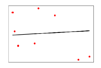
In the above output, we can see the regression line between the data points.

Step 6: Performance computation

We can also compute the performance of our regression model with the help of various performance metrics as follows.

print("Regressor model performance:")print("Mean absolute error(MAE) =",round(sm.mean_absolute_error(y_test, y_test_pred),2))print("Mean squared error(MSE) =",round(sm.mean_squared_error(y_test, y_test_pred),2))print("Median absolute error =",round(sm.median_absolute_error(y_test, y_test_pred),2))print("Explain variance score =",round(sm.explained_variance_score(y_test, y_test_pred),2))print("R2 score =",round(sm.r2_score(y_test, y_test_pred),2))

Output

Regressor model performance:
Mean absolute error(MAE) = 1.78
Mean squared error(MSE) = 3.89
Median absolute error = 2.01
Explain variance score = -0.09
R2 score = -0.09